交流波形観測の電圧測定

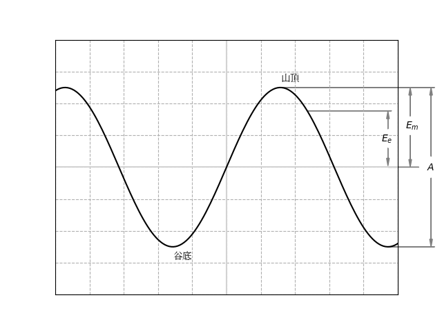
　振幅値と実効値の関係を実験します．

import numpy as np
import matplotlib.pyplot as plt

plt.rcParams['font.family'] ='Yu Mincho'

x = np.linspace(-np.pi*2, np.pi*2, 200)

fig = plt.figure()
ax = fig.add_subplot(1, 1, 1)

plt.xticks(np.arange(-5, 6, 1), c='None')
plt.yticks(c='None')
plt.xlim(-5, 5)
plt.ylim(-2.0, 2.0)
plt.grid(ls='--')
plt.axhline(0, c='lightgray')
plt.axvline(0, c='lightgray')
plt.tick_params(length=0)
plt.plot(x, np.sin(x)*1.25, c='k', ls='-')

x90  =  90*np.pi/180
x270 = 270*np.pi/180

ax.text( x90,  1.35, '山頂', fontsize=10)
ax.text(-x90, -1.45, '谷底', fontsize=10)

ax.arrow(x90 ,  1.25, 4.5, 0, color='gray', clip_on=False)
ax.arrow(x270, -1.25, 4.5-np.pi, 0, color='gray', clip_on=False)
ax.arrow(x90+4.4,  0.17, 0,  1.25-0.17, head_width=0.08, length_includes_head=True, color='gray', clip_on=False)
ax.arrow(x90+4.4, -0.17, 0, -1.25+0.17, head_width=0.08, length_includes_head=True, color='gray', clip_on=False)
ax.text(x270+1.14, -0.05, '$\it{A}$')

ax.arrow(x270, 0, 0.9, 0, color='gray', clip_on=False)
ax.arrow(x270+0.65, 0.8, 0, 1.25-0.8, head_width=0.08, length_includes_head=True, color='gray', clip_on=False)
ax.arrow(x270+0.65, 0.5, 0, -0.5,     head_width=0.08, length_includes_head=True, color='gray', clip_on=False)
ax.text(x270+0.5, 0.6, '$\it{E_m}$')

x2 = np.arcsin(1/np.sqrt(2))
ax.arrow(x90+x2, 1.25/np.sqrt(2), np.pi-x2+0.1, 0, color='gray', clip_on=False)
ax.arrow(x270, 0.6, 0,  0.28, head_width=0.08, length_includes_head=True, color='gray', clip_on=False)
ax.arrow(x270, 0.3, 0, -0.28, head_width=0.08, length_includes_head=True, color='gray', clip_on=False)
ax.text(x270-0.2, 0.4, '$\it{E_e}$')

plt.show()

volt.py

clip_on=False で 枠外に描画します．ほかにいい方法があれば教えてください．